
Demand-Driven Performance FAQ
Providing customers what they need, when they need it, while lowering the overall cost of delivery and improving ROI
06.1 Configure And Manage Supply Chains To More Effectively Address The Challenges Associated With Inventory Management (Part 1 of 3) (DDPSC06.1)
06a. How do we nullify the effects of variability in supply to improve inventory performance?
The best way to nullify the effects of variability, whether on the supply-side or demand-side, is to contain the variability. In DDPSC02, Identifying and Addressing Organizational Measurements, we identified the most significant effect of variability to be time delays in processing that result in a time delay in satisfying demand. Therefore, we should examine the time to re-supply that we are using when replenishing inventory buffers to see if it will actually contain the variability on the supply side. If you look at the data that you have in hand, what you will likely find is that the overall time to complete a number of work orders for any given item varies with some sort of a distribution between the longest and shortest time required, and a corresponding average.

ddpsc06.1 figure 1 - using an average lead-time means 50% of the time, supply-side variability is not contained
When we think about containing supply-side variability, it becomes quite clear that using an average lead-time will leave us in a position where 50 percent of the time the supply-side variability will not be contained. When actual lead times exceed planned lead times, we either deliver late (whether we are supplying a customer directly or re-supplying an inventory buffer), or we expedite (expending more resources in terms of overtime and premium freight) in an effort to compensate for the delays. The simplest solution is to shift our thinking from using an "average" lead-time to a "reliable" lead-time.
A Reliable Lead Time (RLT) would be a planned period of time between the start and finish of an order that is very often greater than and seldom less than the actual time required for each individual order to be completed. Depending on your business, a RLT could be set to cover 90 or 95 percent of the variability, or as much as 100 percent if delivering on-time or ensuring inventory buffers never yield an out-of-stock condition, provides a competitive advantage.
When re-supplying a replenishment based inventory buffer, the RLT is often referred to as the Time to Reliably Replenish (TRR).

DDPSC06.1 FIGURE 2 - USING A RELIAGLE LEAD TIME (RLT) MEANS COVERING THE SPREAD OF PLANNED VS. ACTUAL LEAD TIMES, SO THAT SUPPLY-SIDE VARIABILITY IS CONTAINED
If the RLT required to provide customers with reliable promised delivery dates is longer than customers' are willing to wait, then you will have to address the underlying causes of supply-side variability, some of which could be organizational misalignments (DDPSC04), rather than simply using the RLT to contain the variability.
06b. How do we nullify the effects of variability in demand to improve inventory performance?
Now that we understand how to contain supply-side variability, we can turn our attention to sizing inventory buffers to contain demand-side variability. What you see depicted below is an example of what customer demand, or, better yet, Point Of Sale (POS) demand looks like on a day-to-day basis, or in any other time interval. This could be historical or forecasted demand, whichever best represents the type of demand you would expect to be buffering.

ddpsc06.1 figure 3 - point of sale (pos) demand on day-to-day basis
Utilizing the Reliable Lead Time (RLT) information we determined previously, we can now view at the item (i.e., Part Number (PN) or Stock Keeping Unit (SKU)) level, how this daily demand accumulates in windows of RLT.
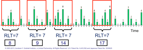
ddpsc06.1 figure 4 - examining pos demand to contain demand-side variability
The cumulative demand in each window of RLT can then be displayed on the same time line as the original demand to produce what we call a Time Based Demand Pattern.

ddpsc06.1 figure 5 - an example of a time-based demand pattern
The result is a single picture in which relationships and tradeoffs between supply-side variability, demand-side variability, investments in inventory buffers, and the risk of being out-of-stock can be easily understood and evaluated at the item (i.e., Part Number (PN) or Stock Keeping Unit (SKU)) level throughout an entire supply chain.
Access to this type of information throughout the supply chain clearly requires a certain level of collaborative data exchange that is most effective when it includes reliable POS demand data, and Times to Reliably Replenish for the inventory buffers.
06c. Do changes in the Time to Reliably Replenish (TRR) always result in changes in the size of an inventory buffer?
A linear relationship does not always exist between TRR and inventory buffer size. It is a misnomer to assume that changes in TRR automatically result in changes in the size of the corresponding inventory buffers. The relationship between changes in TRR and changes in the size of the corresponding inventory buffers approaches a one-to-one relationship only as the demand becomes more uniform in quantity and more regular in timing. Even then, the relationship between changes in TRR and changes in the size of the corresponding inventory buffers, cannot be assumed to be one-to-one, but must be computed.

ddpsc06.1 figure 6 - an example of demand uniform in quality and regular in timing

ddpsc06.1 figure 7 - an example of demand uniform in quantity and irregular in timing

ddpsc06.1 figure 8 - an example of demand non-uniform in quantity and regular in timing

ddpsc06.1 figure 9 - an example of demand non-uniform in quantity and irregular in timing
Recall that the size of the inventory buffers is a result of determining the cumulative demand in windows of TRR along a time line. As such, irregular timing in demand changes the cumulative demand in some TRR windows and creates larger time gaps between some TRR windows. Whereas, non-uniform demand, with its highs and lows in demand quantities, will simply change the cumulative demand in some TRR windows. In any event, sizing item (i.e., Part Number (PN) or Stock Keeping Unit (SKU)) level inventory buffers using TRRs with demand that is uniform or non-uniform, regular or irregular, is best accomplished using the methodology described above. For a more comprehensive overview of how properly located and sized inventory buffers can improve availability, reduce out-of-stocks and increase inventory turns, please view: TOC for Inventory Management – Overview.
Next: Configure and Manage supply chains to more effectively address the challenges associated with Inventory Management (DDPSC06.2)
- How would this approach work when sizing buffers for a new product launch, for which there is no history?
- How does TOC use inventory positioning to address the uncertainties of customer demand?
Comments or questions? Email us at info@goldratt.com.